I recently rigged up These Nebulae Do Not Exist. The website shows GAN-generated images of nebulae every time the page is refreshed:
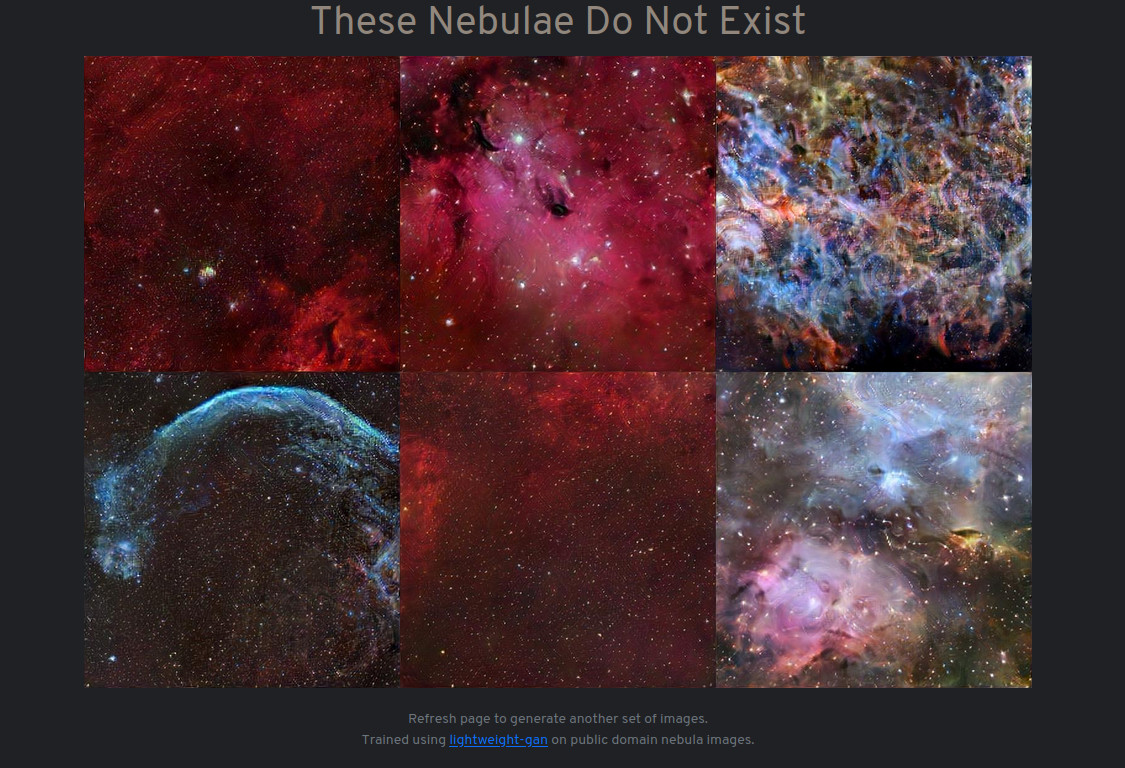
Screenshot of These Nebulae Do Not Exist
In this post, I cover how I assembled it end-to-end, from data scraping, to model training, and finally deploying it as a web app using free services only.
Introduction
Nebulae are my favourite astronomical phenomena. Distant clouds of stardust arrayed like cosmological flowers against the void of the universe, made visible to us thanks to the stupefying resolving power of our space observatories. Inspired by the launch of the James Webb Space Telescope, and the GAN-powered realistic face generator at thispersondoesnotexist.com, I thought of looking at what GANs can do to generate images of nebulae.
Existing work
Screening for existing work, I found:
pearsonkyle/Neural-Nebulawhich uses DCGAN to generate 128x128 nebula pictures.jacobbieker/AstroGANwhich contains code for a spiral galaxy generator, elliptical galaxy generator, and a 128x128 image generator trained on Hubble space telescope images.
Both repos were last updated in Apr and May 2019 respectively, back before high resolution image synthesis with GANs became commonplace.
Data
Data was scraped from publicly available images hosted by space agencies, mostly from NASA, ESA and ESO. Selenium was used to load search results from their image archives, then BeautifulSoup was used to pick out download links from individual image pages.
When skimming through the scraped images, I noticed that the images scraped have varying size and perspecive. Some images show a segment of space where the nebulae is a small object instead of being the focal point of the image. Some images are much longer than they are wide. Some images have pretty high resolution and need to be downsized (e.g. image width and height near ~8000 pixels)
I ended up manually inspecting images in the dataset one by one and preprocessed them as necessary.
- Images that didn’t fit what I wanted were discarded.
- Photos too large to work with are downsized using GIMP, with image sharpening masks applied in moderation.
- Images that had a lot of empty space were cropped into smaller individual images that focused on interesting nebulae features.
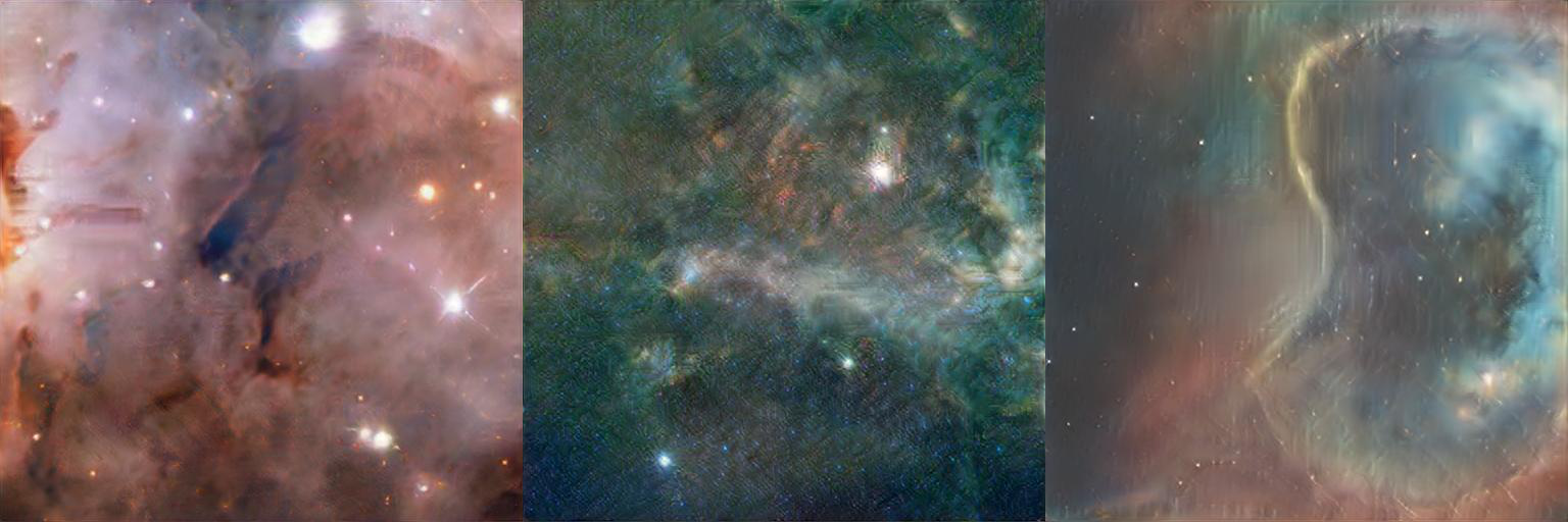
- Composite images that have image-stitching artifacts were cropped to remove blank regions in the image (see example below). If left unattended, generators eventually learnt to produce images with similar stitching artifacts to fool discriminators.
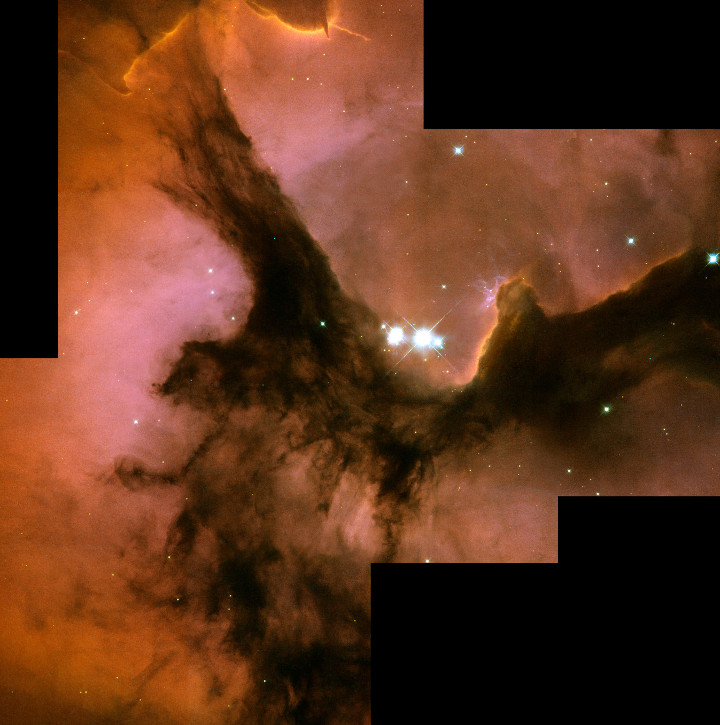
Example image with stitching artifacts. Full HST WFPC2 image of Trifid Nebula. Source: ESA/Hubble
By the time I was done, I had a vetted dataset of ~2k images. At this point, the images have a diverse range of resolutions and aspect ratios thanks to the preprocessing. However, most GANs only work with generating square images. Conventionally, one would simply resize the images to the target resolution, but I opted instead to sample random crops at 512x512 resolution to prevent introducing distortions.
Training
I adopted a lightweight GAN architecture from Towards Faster and Stabilized GAN Training for High-fidelity Few-shot Image Synthesis by Liu et al, implemented in lucidrains/lightweight-gan by the same person who made thispersondoesnotexist.com. Paraphrasing the paper’s summary, this lightweight GAN’s main value proposition is its low computational and data sample requirements, enabling high resolution GAN models to be trained on consumer GPUs within hours, using a small amount of images. This is great as I plan to rely on my personal workstation for training.
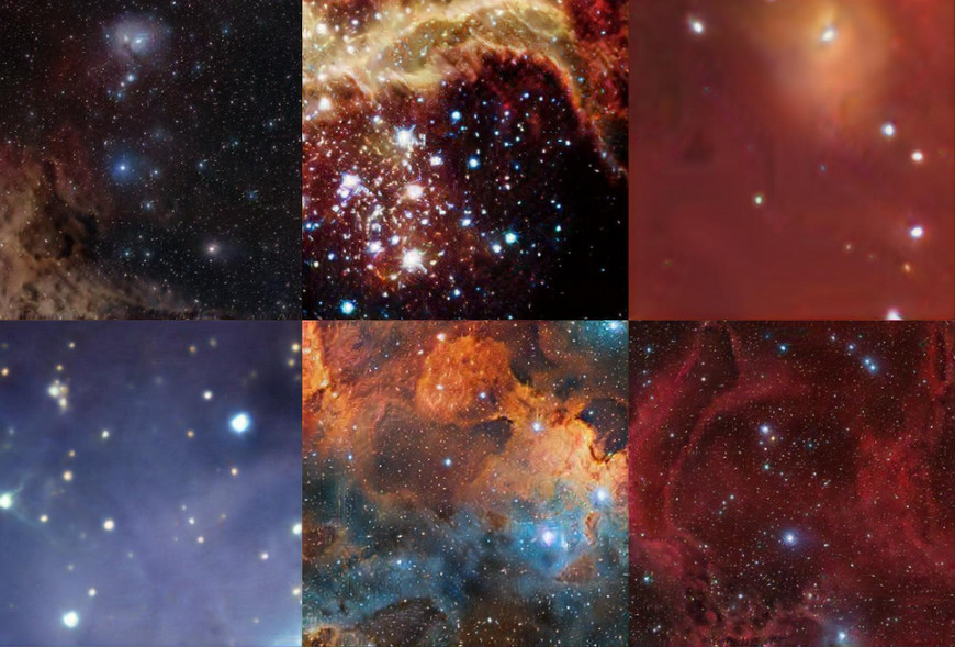
I experimented with the training configuration for a couple of weeks. Overall I was pleased with the results; the images generated were sufficiently realistic and exhibited a diverse range of modalities. Examples below:
Example GAN output 1 Example GAN output 2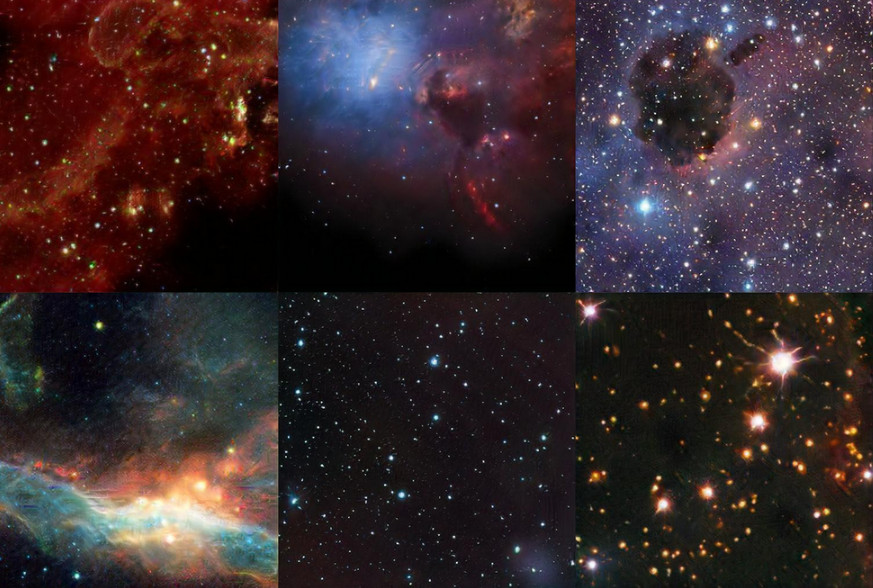
However, every now and then, the generated images exhibit texture artifacts that proved to be difficult to remove despite further experimentation.
Examples of GAN texture artifacts. You might need to open the image in a new tab and zoom in to see it
I eventually concluded that the lightweight GAN architecture has reached its limits, and I’ve reaped all the benefits for something that trains this fast. Using GaParmar/clean-fid, the final model has an FID score 1 of 52.86. For context, Liu et al’s model scored 52.47 FID when trained on 2k images of nature photographs, which places us in a similar ballpark for performance (see table reproduced below).
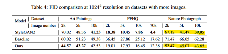
FID scores of Liu et al’s architecture with varying amounts of data, reproduced from their paper. Highlight emphasis mine.
(Not) experimenting with StyleGAN (yet)
At time of writing, the StyleGAN series of models is one of the most well known architectures for generating high fidelity images. According to paperswithcode.com, StyleGAN2 ranks near the top in benchmarks for unconditional image generation and is pretty close to state of the art. The latest iteration is StyleGAN3 released in Oct 2021, which I eagerly adopted to try for this dataset.
Since I was using my personal workstation, model training is progressing rather slowly. According to StyleGAN3 documentation, fully training a model on the FFHQ dataset at 1024x1024 resolution require 5 days 8 hours 2 on 8 V100 GPUs. Given that a p2.8xlarge instance on AWS EC2 with that many GPUs costs 7.2 USD/hr, a single training run on a VM would have cost me ~900 USD. And that’s just base StyleGAN2 without the additional improvements from StyleGAN3; training StyleGAN3-T or StyleGAN3-R would have cost 1.5k USD 3 and 1.8k USD 4!
Given that StyleGAN uses a monstrous amount of compute that I’m not willing to pay for, I’m happy to slowly chip at it on a single GPU over time. This arrangement however places architectural improvements out of immediate reach; practically speaking I would only see returns for experimenting with StyleGAN3 after doing another (or another two) side projects.
I wasn’t keen on waiting that long, and thus as dictated by the project management triangle, once cost and time is prioritized, scope has to give way. The current model has some flaws, but it makes sense to move ahead with deployment and revisit this in the future.
Model export
My first thought was to export the trained generator as an ONNX model. Conventionally, the main use case for exporting to ONNX is to allow model inferencing on a wide variety of languages via the ONNX runtime. In this case, exporting to ONNX is useful because the ONNX runtime in Python only requires protobuf and numpy, allowing a lean, Pytorch-less environment to be used in deployment.
ONNX export relies on first JIT-serializing the model to Torchscript, an intermediate representation of a Pytorch model. This can be done via either scripting or tracing. In scripting, model logic is faithfully replicated from source code. In tracing, a dummy input is forward propagated through the model. The operations that took place are then observed and recorded by Pytorch. Scripting tends to be preferred since it fully represents the model’s control flow, while tracing only records the control flow path taken when using the dummy input. However, scripting requires converting each model operation to a Torchscript counterpart; models with unsupported operations cannot be scripted. (I recommend this blogpost for further reading on this topic.)
Model export went smoothly using torch.onnx.export. I wasn’t able to first convert the model to Torchscript using scripting, so I exported to ONNX using tracing instead. Upon comparison with images generated by the original model, the ONNX-exported model generated images are slightly different from the original model. In other words, the exported model was slightly different from the original model. There were dynamic control flow statements that wasn’t adequately represented using tracing. I wouldn’t mind if the different images looked better, but I prefer the output of the original model.
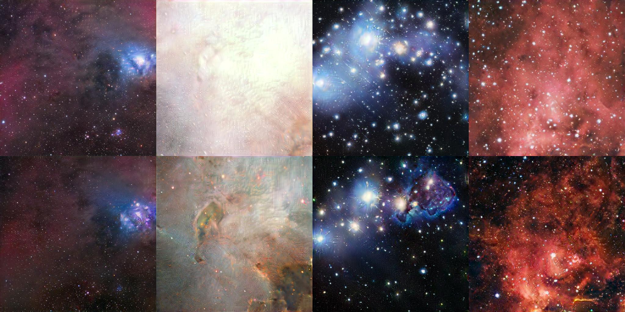
Comparison of images generated by ONNX-exported model (top) vs original Pytorch model (bottom)
I modified the source code to remove blockers for scripting. They were small logical changes like replacing list unpacking with explicit indexing, and replacing lambda functions. I stopped when Pytorch complained about the use of einops.rearrange, which accepts an arbitrary amount of function arguments:
NotSupportedError: Compiled functions can't take variable number of arguments
or use keyword-only arguments with defaults:
  File "/home/tnwei/miniconda3/envs/gan/lib/python3.9/site-packages/einops/
  einops.py", line 393

def rearrange(tensor, pattern: str, **axes_lengths):
                                     ~~~~~~~~~~~~~ <--- HERE
    """
    einops.rearrange is a reader-friendly smart element reordering for
    multidimensional tensors.
einops is a useful package that allows expressing complex tensor manipulation in declarative Einstein notation. At time of writing, einops functions have yet to support scripting to Torchscript according to this github issue. Enabling scripting for the trained generator would require me to replace all calls to einops with equivalent logic. Under any circumstance but this, I’m a huge fan of the package. But in this scenario, untangling elegant Einstein notation like (b h) (x y) d -> b (h d) x y into corresponding torch.reshape’s and torch.permute’s is too much for a Saturday afternoon.
I decided to just extract the trained generator’s state_dict and its source code for inferencing using Pytorch.
Deployment
The end product of this work is envisioned to be a simple website that shows a new generated image upon page refresh. I went ahead and cobbled together a simple FastAPI app packaged in a Docker container that serves a generated image in a static HTML landing page. On my workstation with a 6-core Ryzen 5 3600 CPU, generating a new image takes ~1 second on average.
I imagine someone visiting the site would not want to wait long to see another image when refreshing the page. Thus for good user experience, I need to reduce page refresh latency to at least a few hundred milliseconds. Thanks to the extra moments thinking about cost (see previous section), I’ve also made up my mind to only use free resources for this side project. In other words, deployment options are limited to cloud free tier limits. Thus, renting powerful compute is out of the question, GPU-accelerated or not. Latency is an issue that will need to be resolved without scaling compute.
It eventually occured to me that the fastest way to generate an image is to load one that already exists. The website can load pre-generated images from object storage, which is routinely topped up with model inferencing running in background workers. Effectively, the wait time for generating images is hidden from the end user, as long as the store of pre-generated images is not fully depleted. If the pre-generated images run out, the user will need to wait for the backend to directly generate a new image, which honestly isn’t the end of the world for a side project like this. Sounds like a plan.
Major cloud providers are not keen on giving you an always-free-tier VM. For context, AWS only makes the t2-micro and t3-micro instances available for this purpose, they come with either 1 or 2 vCPUs and a measly 1GB RAM, and will be performance-throttled if you’re using them too much. By contrast, they are much more generous with their serverless services. Google Cloud Run and Azure Container Apps allow running containerized applications within an always-free-tier usage quota 5. Given that my web app doesn’t need to be stateful, a serverless architecture is fair game. Between GCP and Azure, I chose to go with Cloud Run since I’ve seen more mentions of it on the internet compared to Container Apps.
The complete application architecture diagram is as follows:
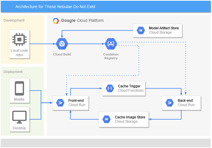
The existing FastAPI web app is split into a light frontend that only serves the HTML page, and a relatively heavy backend that only generates images. When called, the frontend serves the landing page using the oldest image from the bucket. Once served, a Cloud Function calls the backend to generate a new image to replace the image that was just displayed. If multiple calls to the frontend are made in quick succession, Cloud Run will start up additional backend instances to cater for the increase in load.
It takes an average of ~7 seconds for the backend to generate and return a new image. Thanks to how the application architecture is set up, the frontend only needs an average of 310 ms to load the image from object storage, which fits my requirements.
The final step for deployment is to set up a vanity URL redirecting to the Cloud Run frontend. Sticking to my guns on using free resources only, I used a cheeky iframe to embed the server-rendered front end in my static github.io personal site.
Conclusion and further thoughts
You might be surprised to hear that throughout this project, dataset curation easily took the most time and manual effort. I think it was well worth the effort; I doubt GAN training would have went as smoothly if I just dumped the scraped output directly into model training.
Personally I’m not satisfied with the quality of the images generated; I think there is definitely room for improvement. I do plan to update the deployed model if further experimentation bears fruit.
This project stands on the shoulders of giants. Its building blocks exist thanks to the rapid advances of ML research, the rise of skilled ML research engineers implementing user-friendly training codebases, and the proliferation of cloud services. If we rewind the clock by a couple of years, it would not have been possible to complete this project with the level of effort I put into it. These good people have my gratitude.
FID represents Fréchet inception distance, a metric for similarity between generated images and actual images. Lower is better. Wikipedia link ↩︎
Time to fully train StyleGAN2: 17.55 s/k-imgs * 25000 k-imgs * 1.05 ~= 460k seconds ~= 5d 8h. ↩︎
Time to fully StyleGAN3-T: 28.71 s/k-imgs * 25000 k-imgs * 1.05 ~= 754k s ~= 8d 17h. Times 7.2 USD/hr gives 1505 USD. ↩︎
Time to fully train StyleGAN3-R: 34.12 s/k-imgs * 25000 k-imgs * 1.05 ~= 754k s ~= 10d 9h. Times 7.2 USD/hr gives 1793 USD. ↩︎
I was surprised to find that AWS Fargate has no free-tier usage quota. ↩︎